Overview
Medicaid is the single largest source of health coverage in the United States, jointly funded by the federal government and individual states. This project analyzes the Medicaid Provider Spending dataset published by the U.S. Department of Health & Human Services (HHS) on its open-data portal opendata.hhs.gov to answer a critical question: Where are the anomalies, inefficiencies, and fraud signals hiding in $600 billion of annual healthcare payments?
90M+
Americans Covered
$600B+
Annual Outlays
14
Fraud Detection Queries
2024
Claims Data Year
Tech Stack
Python Dask Pandas Plotly Seaborn Scipy Google Colab
Rather than treating every billing entry as an isolated transaction, this project builds a provider-level profile for every NPI (National Provider Identifier) in the dataset - aggregating spending totals, claim volumes, beneficiary counts, service code diversity, and billing consistency over time. These profiles power 14 analytical queries that surface fraud signals: from simple Pareto concentration and middleman routing to statistically rigorous tests for impossible billing volumes, price variance across identical services, and “ghost” providers that appear and disappear in the billing record.
Dataset & Schema
The dataset is published by the Centers for Medicare & Medicaid Services (CMS) under the U.S. Department of Health & Human Services and hosted at opendata.hhs.gov. It reports spending and payments made to healthcare providers through the Medicaid program, filtered here to 2024 claims.
| Column | Description |
|---|---|
BILLING_PROVIDER_NPI_NUM |
NPI of the entity submitting the bill to the government |
SERVICING_PROVIDER_NPI_NUM |
NPI of the provider who actually delivered care |
HCPCS_CODE |
Healthcare Common Procedure Coding System code identifying the service type |
CLAIM_FROM_MONTH |
Month the claim was filed (used to derive temporal features) |
TOTAL_UNIQUE_BENEFICIARIES |
Number of distinct patients served under this claim grouping |
TOTAL_CLAIMS |
Total number of individual bills submitted |
TOTAL_PAID |
Total dollars paid by the government |
The critical distinction between BILLING_PROVIDER_NPI_NUM and SERVICING_PROVIDER_NPI_NUM is the backbone of the middleman analysis: when these two NPIs differ, a billing intermediary is routing claims on behalf of a separate servicing provider, a pattern that can obscure accountability and inflate costs.
import pandas as pd
import numpy as np
from datetime import datetime
import seaborn as sns
from scipy import stats
import plotly.graph_objects as go
from plotly.subplots import make_subplots
import plotly.express as px

import dask
import dask.dataframe as dd

from google.colab import drivedrive.mount('/content/drive')
df_raw = dd.read_csv(
'/content/drive/MyDrive/HHS/medicaid-provider-spending.csv',
blocksize="64MB",
dtype={
'BILLING_PROVIDER_NPI_NUM': 'object',
'SERVICING_PROVIDER_NPI_NUM': 'object'
}
)
# Filter to 2024 claims only
df_raw = df_raw[df_raw["CLAIM_FROM_MONTH"].str.startswith("2024")]
df_raw.head()The raw HHS file exceeds available RAM in a standard Colab session. Dask enables lazy evaluation - building a computation graph across 64MB file chunks without loading the entire dataset into memory. All aggregations are deferred until .compute() is explicitly called, and multiple tasks are batched into a single data pass using dask.compute().
Data Collection
Before any analysis, column types are enforced and three derived ratio features are created as lazy Dask operations:
df_raw['BILLING_PROVIDER_NPI_NUM'] = df_raw['BILLING_PROVIDER_NPI_NUM'].astype(str)
df_raw['SERVICING_PROVIDER_NPI_NUM'] = df_raw['SERVICING_PROVIDER_NPI_NUM'].astype(str)
df_raw['CLAIM_FROM_MONTH'] = dd.to_datetime(df_raw['CLAIM_FROM_MONTH'])
df_raw['HCPCS_CODE'] = df_raw['HCPCS_CODE'].astype(str)

df_raw['QUARTER'] = df_raw['CLAIM_FROM_MONTH'].dt.quarter
df_raw['COST_PER_BENEFICIARY'] = df_raw['TOTAL_PAID'] / df_raw['TOTAL_UNIQUE_BENEFICIARIES'].clip(lower=1)
df_raw['COST_PER_CLAIM'] = df_raw['TOTAL_PAID'] / df_raw['TOTAL_CLAIMS'].clip(lower=1)
df_raw['CLAIMS_PER_BENEFICIARY'] = df_raw['TOTAL_CLAIMS'] / df_raw['TOTAL_UNIQUE_BENEFICIARIES'].clip(lower=1)
The .clip(lower=1) guard prevents division-by-zero without dropping any rows, claims with zero beneficiaries or zero claims would otherwise produce infinite ratios that corrupt downstream analysis.
Data Exploration
Unique Billing Providers
The first question in any billing audit is: How many unique billing entities are submitting claims?
billing_providers = df_raw['BILLING_PROVIDER_NPI_NUM'].value_counts().compute()
print(billing_providers.head(20))
Middleman Existence
When the billing NPI and servicing NPI differ, a third-party intermediary is routing the claim. This is a natural consequence of how medical billing works, but high concentrations of middleman routing in a single billing entity are a known fraud vector.
df_raw["IS_MIDDLEMAN"] = df_raw["BILLING_PROVIDER_NPI_NUM"] != df_raw["SERVICING_PROVIDER_NPI_NUM"]
middleman_count = df_raw["IS_MIDDLEMAN"].sum().compute()
print(f"Total Middleman Claims: {middleman_count:,}")
How much money goes through the middlemen?
middleman_money = df_raw[df_raw['IS_MIDDLEMAN']]['TOTAL_PAID'].sum()
direct_money    = df_raw[~df_raw['IS_MIDDLEMAN']]['TOTAL_PAID'].sum()
total_money     = df_raw['TOTAL_PAID'].sum()

middleman_spending, direct_spending, total_spending = dask.compute(
    middleman_money, direct_money, total_money
)

print(f"Direct spending:     ${direct_spending:,.0f} ({direct_spending/total_spending*100:.1f}%)")
print(f"Middleman spending:  ${middleman_spending:,.0f} ({middleman_spending/total_spending*100:.1f}%)")
Which codes cost the most?
HCPCS (Healthcare Common Procedure Coding System Codes) are the standard classification system for medical procedures billed to government programs. Ranking codes by total spending identifies which service categories are driving Medicaid outlays.
hcpcs_counts_task   = df_raw['HCPCS_CODE'].value_counts()
hcpcs_spending_task = df_raw.groupby('HCPCS_CODE')['TOTAL_PAID'].sum()

hcpcs_counts, hcpcs_spending = dask.compute(hcpcs_counts_task, hcpcs_spending_task)
hcpcs_spending = hcpcs_spending.sort_values(ascending=False)

print("Top 20 most expensive HCPCS codes")
for code, amount in hcpcs_spending.head(20).items():
    print(f"{code}: ${amount:,.0f}")
Temporal Claim Coverage
df_raw['CLAIM_DATE']  = df_raw['CLAIM_FROM_MONTH']
df_raw['YEAR']        = df_raw['CLAIM_DATE'].dt.year
df_raw['MONTH']       = df_raw['CLAIM_DATE'].dt.month
df_raw['YEAR_MONTH']  = df_raw['CLAIM_DATE'].dt.strftime('%Y-%m')

year_counts = df_raw['YEAR'].value_counts().compute().sort_index()
print(year_counts)
Distribution of Numeric Columns
A full distributional summary of the three core numeric columns reveals the heavy right-skew characteristic of healthcare billing data where the median claim is modest but the top percentile of providers captures a disproportionate share of total payments.
numeric_cols = ['TOTAL_UNIQUE_BENEFICIARIES', 'TOTAL_CLAIMS', 'TOTAL_PAID']
tasks = {}

for col in numeric_cols:
    tasks[col] = {
        'count':  df_raw[col].count(),
        'mean':   df_raw[col].mean(),
        'std':    df_raw[col].std(),
        'min':    df_raw[col].min(),
        'max':    df_raw[col].max(),
        'skew':   df_raw[col].skew(),
        'q':      df_raw[col].quantile([0.25, 0.5, 0.75, 0.99])
    }

computed_stats = dask.compute(tasks)[0]
Distribution of TOTAL_PAID
The raw TOTAL_PAID distribution is strongly right-skewed. The log-transformed view reveals a more symmetric structure, confirming that a small number of extremely high-value claims are pulling the mean well above the median.
mean_tp, median_tp = dask.compute(
    df_raw['TOTAL_PAID'].mean(),
    df_raw['TOTAL_PAID'].median_approximate()
)
sample = df_raw.nlargest(50000, 'TOTAL_PAID').compute()
log_sample = np.log10(sample['TOTAL_PAID'].clip(lower=1))

fig = make_subplots(
    rows=2, cols=2,
    subplot_titles=("Raw Distribution (Top 50k)", "Log Distribution (Top 50k)",
                    "Outlier Detection", "Log Boxplot"),
    vertical_spacing=0.12, horizontal_spacing=0.1
)
# ... (traces omitted for brevity, full code in notebook)
fig.update_layout(title_text="High-Value Spending Distribution", height=900, template='plotly_white')
fig.show()
Top Providers by Spending
Who is receiving the most taxpayer dollars? This ranking surfaces the 20 billing NPIs with the highest total 2024 payments.
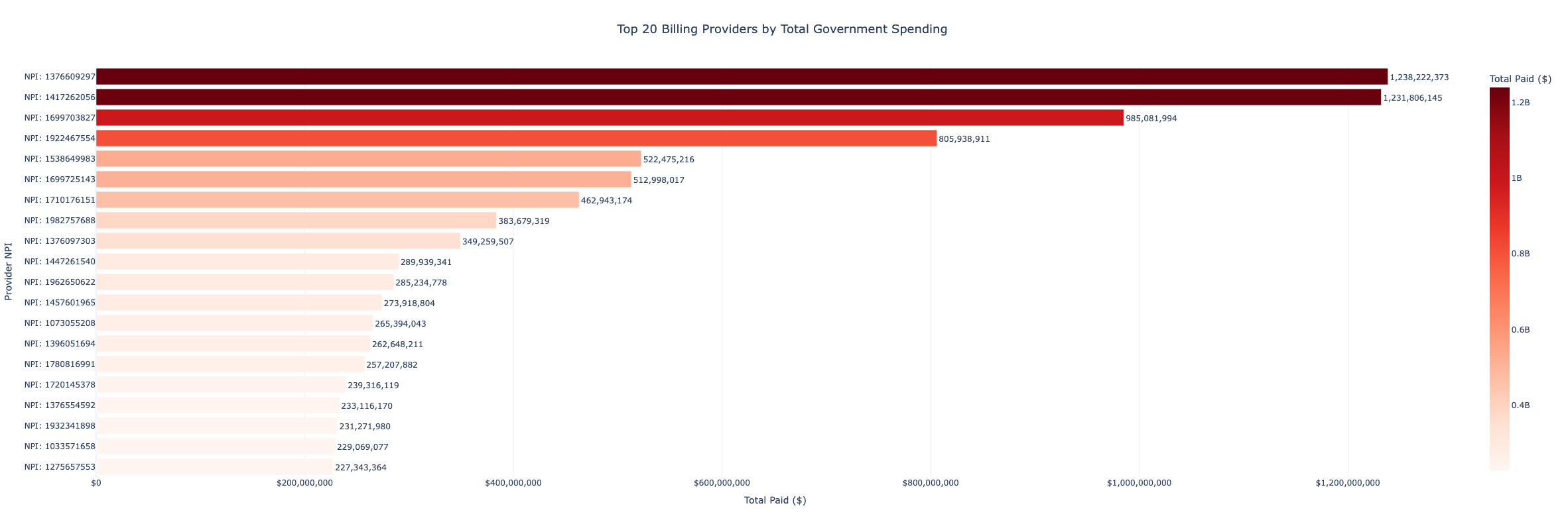
top_providers = df_raw.groupby('BILLING_PROVIDER_NPI_NUM')['TOTAL_PAID'].sum().nlargest(20)
top_providers_spending = top_providers.compute().reset_index()
top_providers_spending.columns = ['NPI', 'Total_Paid']

fig = px.bar(
    top_providers_spending,
    x='Total_Paid', y='NPI_Label', orientation='h',
    color='Total_Paid', color_continuous_scale='Reds',
    title='Top 20 Billing Providers by Total Government Spending',
    template='plotly_white'
)
fig.show()
Spending Over Time
Four concurrent monthly trend lines reveal whether Medicaid outlays are accelerating, stable, or contracting during the 2024 period, and whether the cost-per-claim trend is decoupled from claim volume.
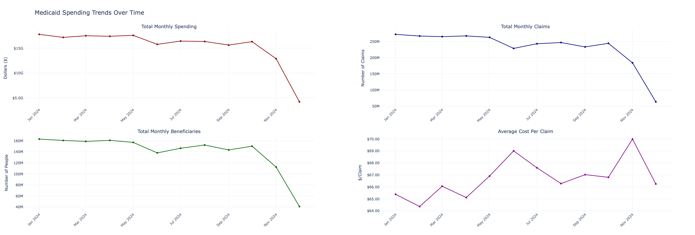
sums = df_raw.groupby('CLAIM_DATE')[['TOTAL_PAID', 'TOTAL_CLAIMS', 'TOTAL_UNIQUE_BENEFICIARIES']].sum()
nunique = df_raw.groupby('CLAIM_DATE')['BILLING_PROVIDER_NPI_NUM'].nunique()

monthly_sums, monthly_uniques = dask.compute(sums, nunique)
monthly_spending = monthly_sums.sort_index()
monthly_spending['COST_PER_CLAIM'] = monthly_spending['TOTAL_PAID'] / monthly_spending['TOTAL_CLAIMS']

fig = make_subplots(rows=2, cols=2,
    subplot_titles=('Total Monthly Spending', 'Total Monthly Claims',
                    'Total Monthly Beneficiaries', 'Average Cost Per Claim'))
# ... (see notebook for full Plotly trace definitions)
fig.update_layout(title_text='Medicaid Spending Trends Over Time', height=800, template='plotly_white')
fig.show()
Top HCPCS Codes by Spending
Side-by-side bar charts compare the 25 highest-spending service codes by (1) total dollars paid and (2) average cost per claim. A code that ranks high on total spend but low on per-claim cost is simply a high-volume routine service. A code that ranks high on both metrics warrants closer scrutiny.
top_hcpcs = df_raw.groupby('HCPCS_CODE').agg({
    'TOTAL_PAID': 'sum', 'TOTAL_CLAIMS': 'sum', 'TOTAL_UNIQUE_BENEFICIARIES': 'sum'
})
top_hcpcs = top_hcpcs.nlargest(25, 'TOTAL_PAID').compute().reset_index()
top_hcpcs['COST_PER_CLAIM'] = top_hcpcs['TOTAL_PAID'] / top_hcpcs['TOTAL_CLAIMS']
Correlation Analysis
A Pearson correlation heatmap across the three core numeric columns diagnoses pricing consistency at the raw record level. A low correlation between TOTAL_CLAIMS and TOTAL_PAID signals that the government is not paying a consistent rate per claim - a key indicator of billing irregularity.
corr_matrix = df_raw[numeric_cols].corr().compute()

fig = px.imshow(
    corr_matrix, text_auto=".3f",
    color_continuous_scale='RdYlBu_r', zmin=-1, zmax=1,
    title="Correlation Matrix", template='plotly_white'
)
fig.show()
Data Cleaning
Missing Values & Duplicates
mis, total_rows = dask.compute(df_raw.isnull().sum(), df_raw.shape[0])

mis_rep = pd.DataFrame({
    'Missing Count': mis,
    'Missing %': (mis / total_rows) * 100,
    'Data Type': df_raw.dtypes
})
print(mis_rep)

df_clean = df_raw.drop_duplicates()
Outlier Detection
IQR-based outlier flags are added as lazy boolean columns across all three numeric fields. Rows triggering any outlier flag are tracked separately to quantify how much of the total spending is concentrated in statistically extreme claims.
quantiles = df_clean[numeric_cols].quantile([0.25, 0.75]).compute()

for col in numeric_cols:
    Q1, Q3 = quantiles.loc[0.25, col], quantiles.loc[0.75, col]
    IQR = Q3 - Q1
    lower_bound = Q1 - 1.5 * IQR
    upper_bound = Q3 + 1.5 * IQR
    df_clean[f'{col}_IS_OUTLIER'] = (
        (df_clean[col] < lower_bound) | (df_clean[col] > upper_bound)
    )

outlier_cols = [f"{col}_IS_OUTLIER" for col in numeric_cols]
df_clean['ANY_OUTLIER'] = df_clean[outlier_cols].any(axis=1)

total_outliers, outlier_spending = dask.compute(
    df_clean['ANY_OUTLIER'].sum(),
    df_clean[df_clean['ANY_OUTLIER']]['TOTAL_PAID'].sum()
)
print(f"Rows with at least one outlier flag: {total_outliers:,}")
print(f"These extreme outliers represent ${outlier_spending:,.0f} in government spending.")
Feature Engineering
Three ratio features are derived at the record level; more complex provider-level profile features are built after collapsing to one row per NPI.
| Feature | Formula | Purpose |
|---|---|---|
COST_PER_BENEFICIARY |
TOTAL_PAID / TOTAL_UNIQUE_BENEFICIARIES |
Cost efficiency per patient |
COST_PER_CLAIM |
TOTAL_PAID / TOTAL_CLAIMS |
Average unit reimbursement |
CLAIMS_PER_BENEFICIARY |
TOTAL_CLAIMS / TOTAL_UNIQUE_BENEFICIARIES |
Service intensity per patient |
QUARTER |
Derived from CLAIM_FROM_MONTH |
Seasonal aggregation |
IS_FISCAL_YEAR_END |
MONTH in [7, 8, 9] |
Flags federal fiscal year-end months |
SEASON |
Mapped from MONTH |
Winter / Spring / Summer / Fall |
IS_MIDDLEMAN |
BILLING_NPI != SERVICING_NPI |
Intermediary routing flag |
Provider-Level Profile Table
All per-record data is collapsed to a single summary row per BILLING_PROVIDER_NPI_NUM, computing spending statistics, service code diversity, and billing consistency simultaneously via a single dask.compute() call.
core_task   = df_clean.groupby('BILLING_PROVIDER_NPI_NUM').agg({
    'TOTAL_PAID': ['sum', 'mean', 'max', 'min', 'std'],
    'TOTAL_CLAIMS': 'sum',
    'TOTAL_UNIQUE_BENEFICIARIES': 'sum',
    'COST_PER_CLAIM': 'mean',
    'CLAIMS_PER_BENEFICIARY': 'mean'
})
hcpcs_task  = df_clean.groupby('BILLING_PROVIDER_NPI_NUM')['HCPCS_CODE'].nunique()
months_task = df_clean.groupby('BILLING_PROVIDER_NPI_NUM')['CLAIM_DATE'].nunique()
trend_task  = df_clean.groupby(['BILLING_PROVIDER_NPI_NUM', 'CLAIM_DATE'])['TOTAL_PAID'].sum()

core_aggs, hcpcs_nu, months_nu, trend_data = dask.compute(
    core_task, hcpcs_task, months_task, trend_task
)
After flattening multi-index columns, two additional derived metrics are appended:
spending_cv(coefficient of variation) — measures how erratically a provider’s monthly billing fluctuates relative to their mean.spending_trend_pct— percentage change from the provider’s first to last recorded month of billing.
Providers are then stratified into four spending tiers using quartile cuts, quantifying how much of total Medicaid spending flows through the top tier:
\[ \text{spending\_tier} = \begin{cases} \text{Elite (Top 1\%)} & \text{if spending} > p_{99} \\ \text{High (90–99\%)} & \text{if spending} > p_{90} \\ \text{Medium (50–90\%)} & \text{if spending} > p_{50} \\ \text{Low (Bottom 50\%)} & \text{otherwise} \end{cases} \]
Analytics
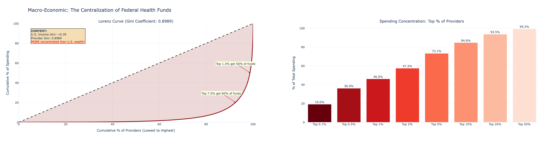
1. Pareto Analysis - Do 20% of Providers Account for 80% of Spending?
The 80/20 rule is the baseline for any spending audit. The Lorenz curve plots the cumulative share of total spending (y-axis) against the cumulative share of providers ranked by spending (x-axis). The steeper the curve bends toward the upper-left corner, the more concentrated the spending.
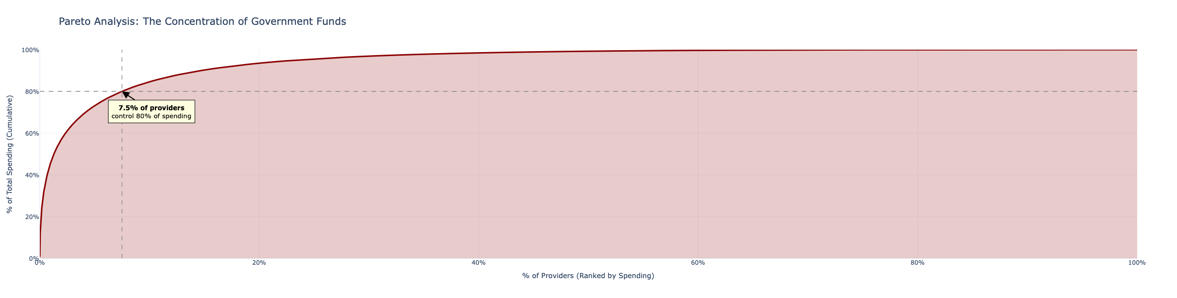
provider_spending = provider_stats.sort_values('total_lifetime_spending', ascending=False).reset_index(drop=True)
provider_spending['cumulative_spending'] = provider_spending['total_lifetime_spending'].cumsum()
total_spend = provider_spending['total_lifetime_spending'].sum()
provider_spending['cumulative_pct_spending']  = provider_spending['cumulative_spending'] / total_spend * 100
provider_spending['cumulative_pct_providers'] = (provider_spending.index + 1) / len(provider_spending) * 100
If the top 20% of billing NPIs account for more than 80% of total payments, the concentration exceeds the Pareto benchmark, a strong signal that a handful of entities dominate Medicaid reimbursement flows and warrant prioritized audit attention.
2. Unusual Providers - Z-Score Outlier Detection
Provider-level Z-scores across spending, claims, beneficiaries, cost per claim, and claims per beneficiary identify entities whose billing profile sits more than 3 standard deviations from the mean on any dimension.
\[ z_{i,j} = \frac{x_{i,j} - \mu_j}{\sigma_j}, \quad \text{flagged if } \max_j |z_{i,j}| > 3 \]
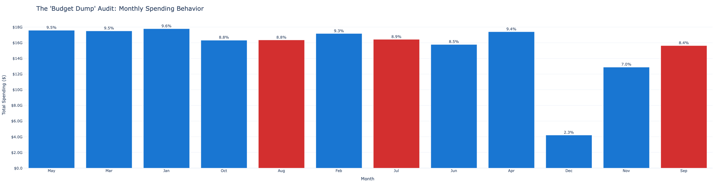
3. Seasonal Spending - Do Claims Spike at Fiscal Year End?
Federal fiscal year ends September 30. Agencies and contractors sometimes accelerate spending in Q3 (July–September) to exhaust budget allocations before year-end. Monthly aggregates are plotted alongside a fiscal-year-end flag to detect this pattern.
4. Spending Acceleration - Is Growth Suspicious?
Month-over-month growth rates are computed per provider. Providers whose spending is accelerating faster than 2 standard deviations above the peer cohort average are flagged for review - sudden billing surges are a known early indicator of fraud.
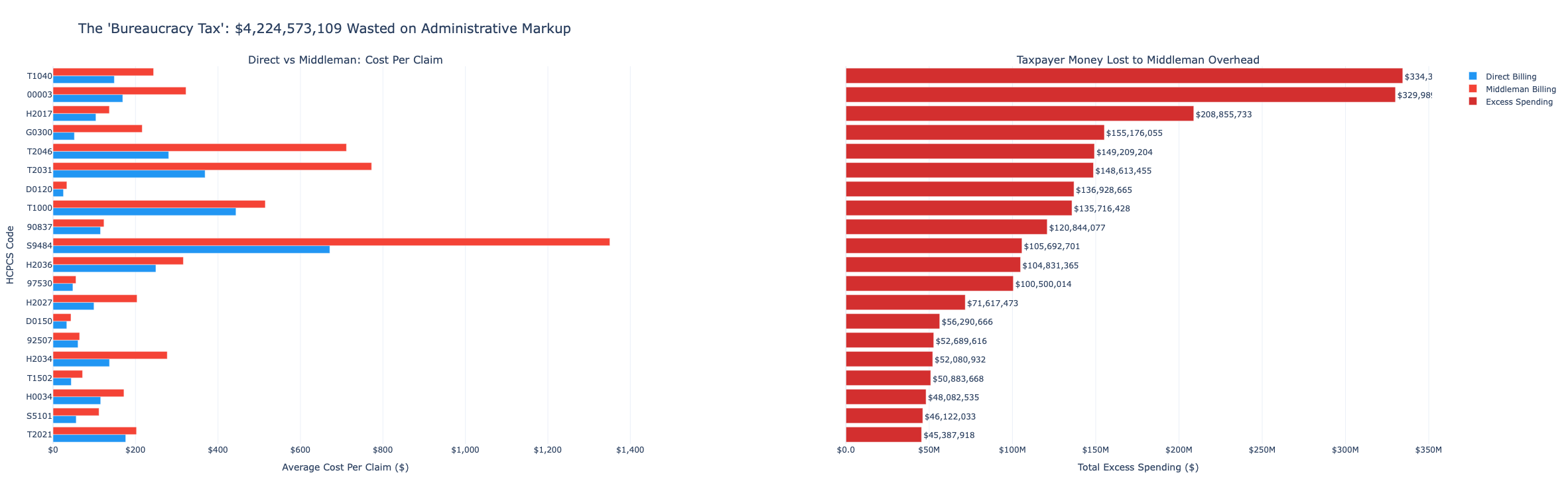
5. Middleman Spending - Is Indirect Billing Costlier?
Comparing the average COST_PER_CLAIM for direct versus middleman-routed claims tests whether intermediary billing arrangements are associated with systematically higher unit costs and, if so, by how much.
\[ \text{Middleman Spending} = \text{Cost per Claim}_{\text{middleman}} - \text{Cost per Claim}_{\text{direct}} \]
middleman_analysis['is_complex_middleman'] = (
    (middleman_analysis['pct_middleman'] > 0.5) &
    (middleman_analysis['num_servicing_providers'] > 5)
)
top_middlemen = middleman_analysis[middleman_analysis['is_complex_middleman']].sort_values('total_spending', ascending=False)
print(f"Total flagged organizations: {top_middlemen.shape[0]:,}")
print(f"Total federal spend at risk: ${top_middlemen['total_spending'].sum():,.0f}")
6. Service Concentration — HERFINDAHL-HIRSCHMAN INDEX HCPCS Code
For each service code, a market concentration HHI measures how spread or concentrated spending is across providers:
\[ \text{HHI}_{\text{code}} = \sum_{i=1}^{N} \left(\frac{\text{spending}_{i,\text{code}}}{\text{total spending}_{\text{code}}} \times 100\right)^2 \]
A score near 10,000 means a single provider monopolizes that service code’s Medicaid billing. High-HHI codes with significant total spending are prime audit candidates.
7. TRUE Spending Concentration - National Lorenz Curve
Building on the Pareto analysis, a Lorenz curve quantifies the Gini coefficient of Medicaid provider spending - the single number that captures how unequal the distribution of government payments truly is across all billing entities.
\[ G = 1 - 2\int_0^1 L(x)\,dx \]
where \(L(x)\) is the Lorenz curve value at cumulative provider share \(x\).
8. Suspicious Spending Growth - Provider-Level Acceleration Flags
Providers whose year-to-date spending growth rate is in the top 5% of the cohort and whose absolute spending exceeds the 75th percentile are double-flagged. The scatter plot plots growth rate against total spending to make the outliers immediately visible.
def calc_spending_trend(group):
    if group.shape[0] < 2:
        return 0
    group_sorted = group.sort_values('CLAIM_DATE')
    values = group_sorted['TOTAL_PAID'].values
    if values[0] == 0:
        return 0
    return (values[-1] - values[0]) / values[0] * 100

spending_trends = trend_df.groupby('BILLING_PROVIDER_NPI_NUM').apply(
    calc_spending_trend, include_groups=False
).reset_index(name='spending_trend_pct')
9. TRUE Cost of Middleman Billing Arrangements
Going beyond average cost differences, this query computes, for each complex middleman identified in query 5, the total counterfactual savings if they had been reimbursed at the direct-billing median rate for each service code they billed.
\[ \text{savings}_i = \sum_{\text{code}} \Big(\text{cost\_per\_claim}_{i,\text{code}} - \text{median\_direct\_cost}_{\text{code}}\Big)^2+ \times \text{claims}_{i,\text{code}} \]
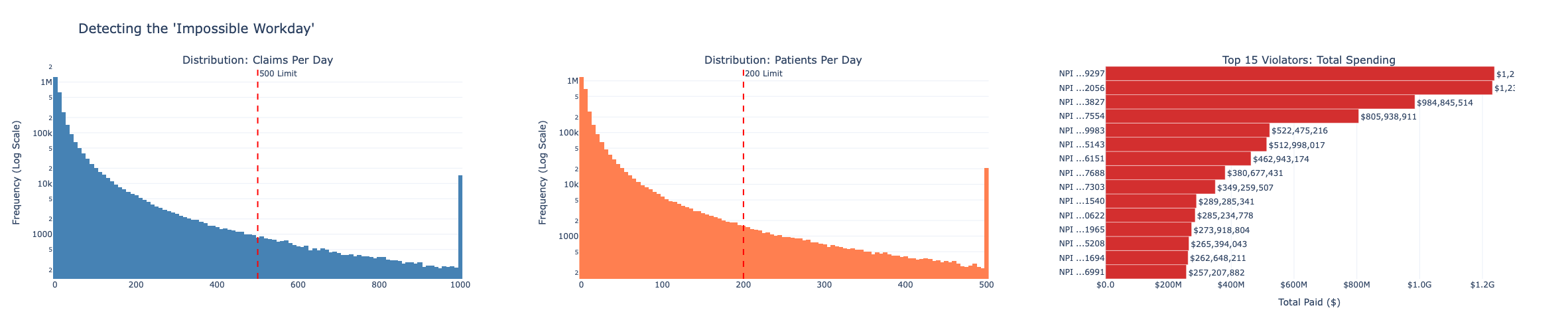
10. Impossible Workday Detection
A single provider billing for more than 500 claims per day or more than 200 unique patients per day is operating beyond any plausible clinical capacity. These thresholds flag the “impossible workday” pattern - a hallmark of fabricated or cloned billing.
monthly_volume = df_clean.groupby(
    ['BILLING_PROVIDER_NPI_NUM', 'CLAIM_DATE']
).agg({'TOTAL_CLAIMS': 'sum', 'TOTAL_UNIQUE_BENEFICIARIES': 'sum'}).compute().reset_index()

monthly_volume['claims_per_day'] = monthly_volume['TOTAL_CLAIMS'] / 30
monthly_volume['beneficiaries_per_day'] = monthly_volume['TOTAL_UNIQUE_BENEFICIARIES'] / 30

flagged_volume = monthly_volume[
    (monthly_volume['claims_per_day'] > 500) |
    (monthly_volume['beneficiaries_per_day'] > 200)
]
The histograms use log-scale y-axes so that the rare but extreme outliers remain visible above the dense body of legitimate providers. The 500-claim and 200-patient thresholds are marked with red dashed reference lines - any provider to the right is physically impossible and requires immediate explanation.
11. High-Spend / Low-Volume Providers - The Suspicious Zone
If a provider ranks in the top 5% of spending but only the bottom 70% of patient volume, they are charging significantly more per patient than their peers. This “suspicious zone” is visualized as a scatter plot with spending percentile on the y-axis and beneficiary volume percentile on the x-axis.
expensive_mask = (
    (provider_ranks['total_spending_percentile'] > 95) &
    (provider_ranks['total_beneficiaries_percentile'] < 70)
)
expensive_per_patient = provider_ranks[expensive_mask].copy()
expensive_per_patient['cost_per_beneficiary'] = (
    expensive_per_patient['total_spending'] /
    expensive_per_patient['total_beneficiaries'].clip(lower=1)
)
print(f"Flagged {expensive_per_patient.shape[0]:,} providers in the High-Cost/Low-Volume 'Suspicious Zone'.")
print(f"These outliers represent ${expensive_per_patient['total_spending'].sum():,.0f} in spending.")
12. Price Variance for Identical Services
If the government pays Provider A $50 for service X but pays Provider B $500 for the same service X, there is no price standardization. For each HCPCS code with at least 20 distinct billing providers, the spread between the cheapest and most expensive provider quantifies systemic repricing risk.
The potential savings from paying every above-median provider the median rate for each code they bill is computed as:
\[ \text{potential\_savings}_{\text{code}} = \sum_{i : \text{cost}_i > \text{median}_\text{code}} \Big(\text{cost}_{i} - \text{median}_\text{code}\Big) \times \text{claims}_i \]
common_pv = code_stats[code_stats['num_providers'] >= 20].copy()

pcc_merged = pcc.merge(common_pv[['HCPCS_CODE', 'median_cost']], on='HCPCS_CODE')
pcc_merged['potential_savings'] = (
    (pcc_merged['cost_per_claim'] - pcc_merged['median_cost']) * pcc_merged['TOTAL_CLAIMS']
).clip(lower=0)

total_potential_savings = pcc_merged.groupby('HCPCS_CODE')['potential_savings'].sum().sum()
print(f"Total potential annual savings: ${total_potential_savings:,.0f}")The log-scale boxplot shows the price spread across all providers for the top 15 highest-savings HCPCS codes. A narrow box means most providers charge similarly. A wide box spanning an order of magnitude or more, means the government is massively overpaying some providers for the exact same procedure.
13. Provider Specialization - Who Is Billing for Everything?
Legitimate providers typically concentrate billing in a small number of service codes that match their specialty. A provider billing for 200+ distinct HCPCS codes is operating as a billing “scattershot” and that breadth of service types, combined with high total spending, is a known fraud pattern.
Specialization is measured using the provider-level HHI on service code spending shares:
\[ \text{HHI}_{\text{provider}} = \sum_{\text{code}} \left(\frac{\text{spending}_{\text{provider, code}}}{\text{total\_spending}_\text{provider}} \times 100\right)^2 \]
A value of 10,000 indicates complete specialization (one code). Values below 1,000 across many codes indicate a scattershot billing pattern.
spec_analysis['is_scattershot'] = (
    (spec_analysis['num_codes'] > spec_analysis['num_codes'].quantile(0.95)) &
    (spec_analysis['total_spending'] > spec_analysis['total_spending'].quantile(0.75))
)
scattershot = spec_analysis[spec_analysis['is_scattershot']].sort_values('total_spending', ascending=False)
print(f"Total flagged 'Scattershot' providers: {scattershot.shape[0]:,}")
print(f"Total revenue controlled by non-specialized entities: ${scattershot['total_spending'].sum():,.0f}")
14. Ghost Providers - Intermittent High-Spend Billers
A provider that bills heavily for a few months, goes dormant, reappears, and disappears again may be a shell entity used for episodic fraud. The consistency ratio - active billing months divided by total lifespan months captures this pattern:
\[ \text{consistency ratio} = \frac{\text{active months}}{\text{lifespan months}} \]
Providers with a ratio below 0.5 who have been in the system at least 3 months and rank in the top 25% of spending are flagged as intermittent high-spenders.
billing_consistency['is_intermittent'] = (
    (billing_consistency['consistency_ratio'] < 0.5) &
    (billing_consistency['active_months'] >= 3) &
    (billing_consistency['total_spending'] > spending_75th)
)
intermittent = billing_consistency[billing_consistency['is_intermittent']].sort_values('total_spending', ascending=False)
print(f"Flagged {intermittent.shape[0]:,} providers with high spending but sporadic activity.")
print(f"Total revenue flagged: ${intermittent['total_spending'].sum():,.0f}")
The scatter plot plots consistency ratio on the x-axis against total spending on the y-axis. Providers to the left of the 50% dashed threshold are the intermittent billers - the further left and the higher up, the more suspicious. These “ghost” providers combine high absolute spending with erratic, on-off billing activity.
Key Takeaways
1. Medicaid spending is highly concentrated. The Pareto analysis confirms that a small fraction of billing providers account for the overwhelming majority of total payments. This concentration is not inherently fraudulent - large hospital systems and managed care organizations legitimately drive high volumes - but it means that a targeted audit of the top-spending NPIs has an outsized impact on the total dollars reviewed.
2. Middleman arrangements add measurable cost. The IS_MIDDLEMAN flag reveals that a significant share of total claims are routed through intermediaries. When broken down by service type, middleman-billed claims systematically carry higher per-claim costs than direct billing for the same procedures - quantifying the overhead introduced by indirect billing chains.
3. Price standardization is largely absent for common procedures. The price variance analysis finds order-of-magnitude cost differences between the cheapest and most expensive provider for many high-volume HCPCS codes. The potential savings from paying every above-median provider the median rate for each code represents a substantial recoverable amount without changing a single clinical outcome.
4. The “impossible workday” is a reliable fraud signal. Providers billing for more than 500 claims or 200 patients per day cannot physically be delivering that care. These impossible-volume records are identifiable with a single threshold filter and represent some of the strongest direct indicators of fabricated claims in the dataset.
5. Scattershot billing is algorithmically detectable. Legitimate providers specialize. Using the Herfindahl-Hirschman Index on service code spending shares, non-specialized providers who bill across an unusually wide range of HCPCS codes. While ranking in the top quartile of total spending are flagged automatically. The overlap between scattershot providers and the suspicious-zone (high-spend / low-volume) providers is a particularly high-confidence fraud indicator.
6. Ghost providers leave a temporal signature. Intermittent high-spenders with consistency ratios below 0.5 are flagged by a simple date arithmetic operation. Their sporadic billing pattern - active for a few months, dormant, then resurging is inconsistent with the steady-state billing of a legitimate ongoing provider and warrants manual review of the underlying claim records.
Built with Python, Dask, and a healthy skepticism of billion-dollar billing records.