A deep dive into Instacart’s 3M+ grocery orders — from EDA to Bayesian hierarchical logistic regression and Poisson cart-size forecasting with Stan
Python
Bayesian Statistics
Stan
Data Science
EDA
Analyzing over 3 million Instacart grocery orders to uncover reorder patterns and forecast cart sizes using exploratory data analysis, feature engineering, and hierarchical Bayesian modeling.
Author
Sailaxman Kotha
Published
October 15, 2025
Overview
Note👨💻 Source Code & Models
The complete Jupyter notebooks, Stan scripts, and raw data are available in the public repository
Instacart is an American grocery delivery platform with millions of users. This project analyzes a sample of over 3 million grocery orders from more than 200,000 users to answer two questions: Which products will a customer reorder? and How many items will they put in their next cart?
Rather than treating every user and product identically, two Bayesian models tackle these questions from different angles. A Hierarchical Bayesian Logistic Regression predicts whether a specific product will be reordered by capturing per-user and per-product variation through random effects. A Bayesian Poisson Regression forecasts how many total items a customer will add to their cart, producing full predictive distributions with credible intervals. Both models are implemented in Stan and sampled via MCMC, enabling principled uncertainty quantification that flat machine learning models cannot provide.
Dataset & Schema
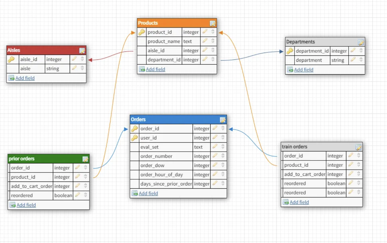
The dataset originates from Instacart’s public release and spans six relational tables. For each user, between 4 and 100 of their orders are available, along with the exact sequence of products added to each cart.
Database schema showing relationships between orders, products, aisles, and departments
NoteKey Tables
orders — All orders (prior, train, test) with timestamps and user info
order_products_prior — Products in each prior order with reorder flags
order_products_train — Products in the most recent order (training target)
products — Product names linked to aisles and departments
aisles & departments — Categorical hierarchies for products
Show code
import pandas as pdimport numpy as npimport seaborn as snsimport matplotlib.pyplot as pltimport plotly.express as pxaisles = pd.read_csv('data/aisles.csv')departments = pd.read_csv('data/departments.csv')order_products_prior = pd.read_csv('data/order_products_prior.csv')order_products_train = pd.read_csv('data/order_products_train.csv')orders = pd.read_csv('data/orders.csv')products = pd.read_csv('data/products.csv')
Data Cleaning & Validation
Before any analysis begins, each of the six tables needs validation for missing values, duplicates, and inconsistent entries.
Missing Values
The days_since_prior_order column contains NaN values — these are not errors. They represent each user’s first ever order, which naturally has no prior order to reference.
Show code
orders.isna().sum()
Duplicate Check & Garbage Values
All tables pass the duplicate check cleanly. Product names, however, contain special characters — accents, hyphens, and symbols — that need normalization.
Show code
import respecial_char =set(re.findall("[^a-zA-Z0-9 ]", ''.join(products.loc[:,'product_name'])))print(f'Found {len(special_char)} distinct special characters in product names')products['product_name'] = products['product_name'].apply(lambda x: re.sub(r'[^a-zA-Z0-9 ]', '', x).strip())
Exploratory Data Analysis
Order Distribution Across Evaluation Sets
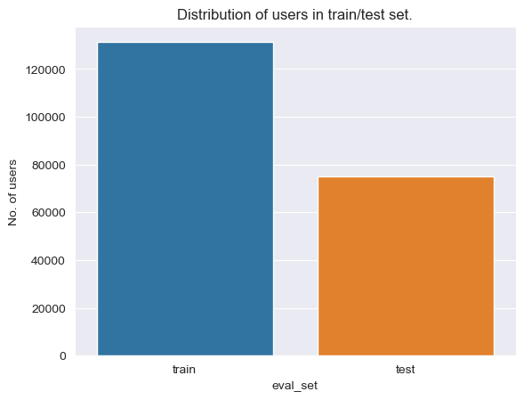
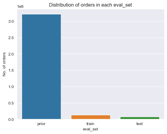
The dataset splits into three evaluation sets. The prior set (3.2M orders) forms the bulk of historical data, while train (~131K) and test (~75K) each represent one user’s most recent order.
Distribution of orders across train and test sets
Distribution across all evaluation sets including prior orders
Reorder vs. First-Time Purchases
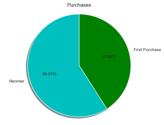
The first critical insight: approximately 59% of all products in orders are reorders. Customers overwhelmingly stick with products they already know.
59% reorders vs 41% first-time purchases
Nearly 6 out of 10 products in any given cart are items the customer has purchased before. This strong reorder tendency makes predicting reorder behavior both feasible and commercially valuable.
Formally, defining \(y_i \in \{0, 1\}\) as the reorder indicator for item \(i\), the overall reorder rate across the dataset is:
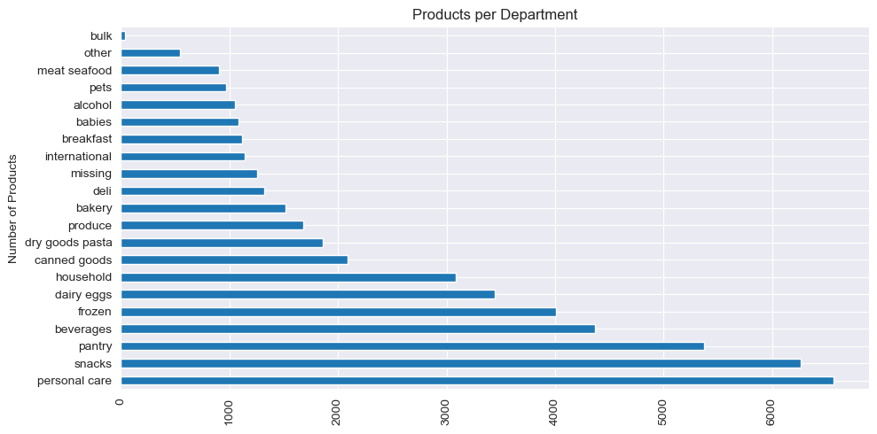
Products span 21 departments. Personal care, snacks, and pantry lead in product count, while categories like bulk and alcohol are smaller and more specialized.
Number of products per department
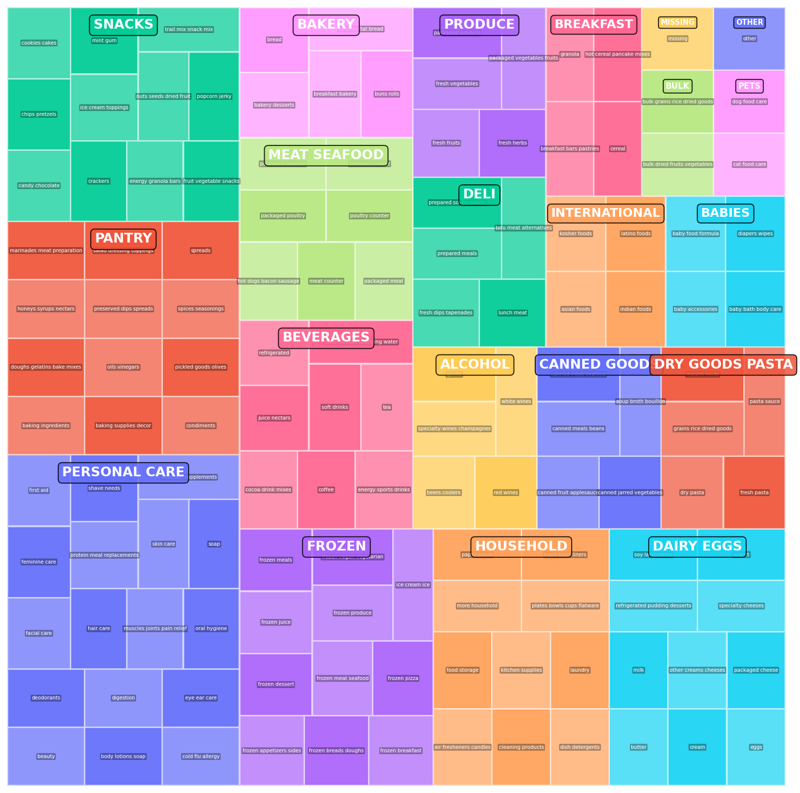
Treemap: Aisles Within Each Department
The hierarchical structure of departments and aisles is best visualized as a treemap. Each rectangle represents an aisle, nested inside its parent department, with area proportional to the number of products. This makes it immediately clear which departments are product-dense and which aisles dominate within them.
Show code
fig = px.treemap(departments_info, path=['department', 'aisle'], title='Aisles in each department')fig.update_layout(autosize=False, width=1050, height=1000)fig.show()
Treemap showing aisles nested within each department — larger rectangles indicate more aisles
Top 15 Departments by Reorder Volume
Ranking departments by total reorder volume (not just rate) reveals which categories generate the most repeat business in absolute terms. This interactive chart highlights the top 15 departments driving habitual purchases.
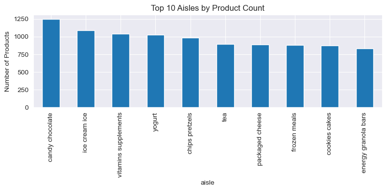
Top Aisles by Product Count
Within departments, the top 10 aisles by product count include candy/chocolate, ice cream, and vitamins/supplements — categories with high product variety.
Top 10 aisles by number of products
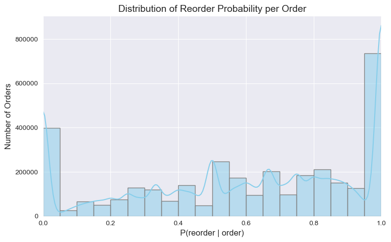
Reorder Rate Distribution
The distribution across orders reveals an interesting shape — most orders cluster around a moderate reorder rate (0.4–0.7), but there is a long tail of orders composed almost entirely of repeat purchases.
Distribution of reorder rates across orders
Deep Dive: Reorder Behavior
Understanding reorder patterns requires slicing the data at multiple levels — department, aisle, time gap, and product.
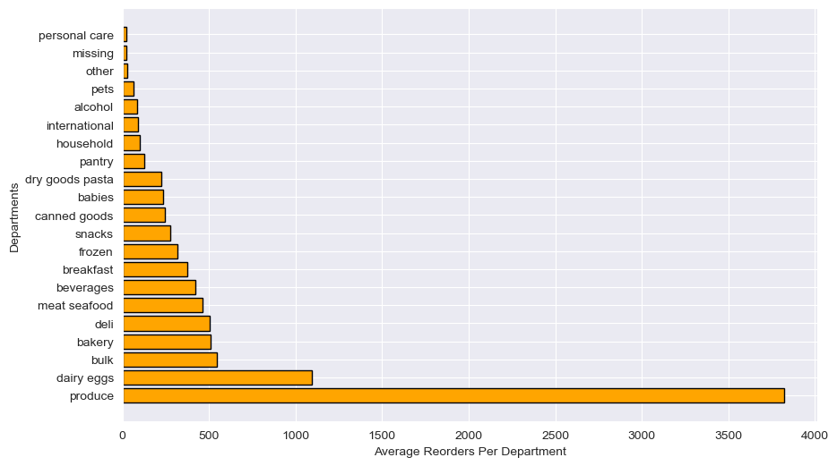
Average Reorders Per Department
Computing the average number of reorders per distinct product in each department highlights which categories drive habitual buying:
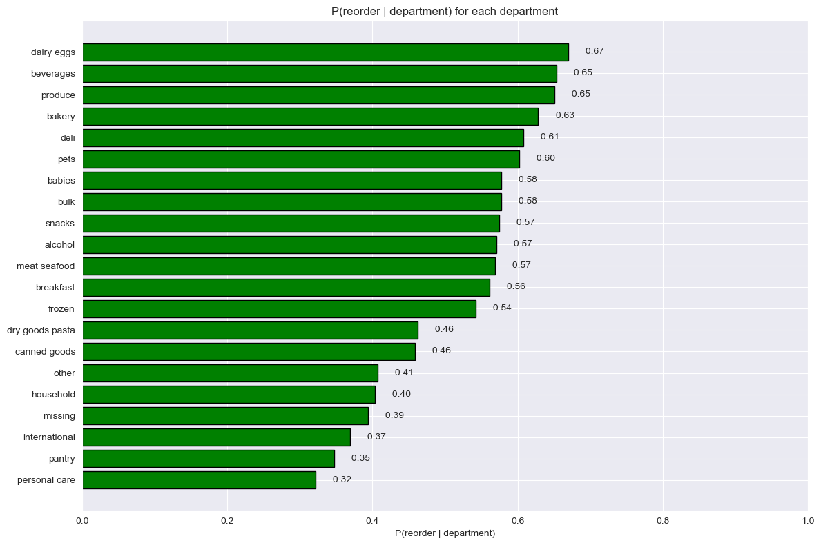
A more informative metric is the conditional probability: “If a product comes from department \(d\), how likely is it to be reordered?”
\[
P(\text{reorder} \mid \text{dept} = d) = \frac{\#\text{reorders from } d}{\#\text{purchases from } d}
\]
Probability of reorder from each department
Show code
dept_probs = departments_info.groupby('department')['reordered'].mean() \ .sort_values(ascending=False)fig, ax = plt.subplots(figsize=(12, 8))bars = ax.barh(dept_probs.index, dept_probs.values, color='green', edgecolor='black')ax.invert_yaxis()ax.set_xlabel('P(reorder | department)')ax.set_title('Reorder Probability by Department')plt.tight_layout()plt.show()
TipHighest Reorder Rates
Dairy & eggs, produce, and beverages show the highest reorder probabilities — staple categories that customers replenish on a regular cycle. The lowest reorder rates appear in personal care and babies, where products tend to be one-time or infrequent purchases.
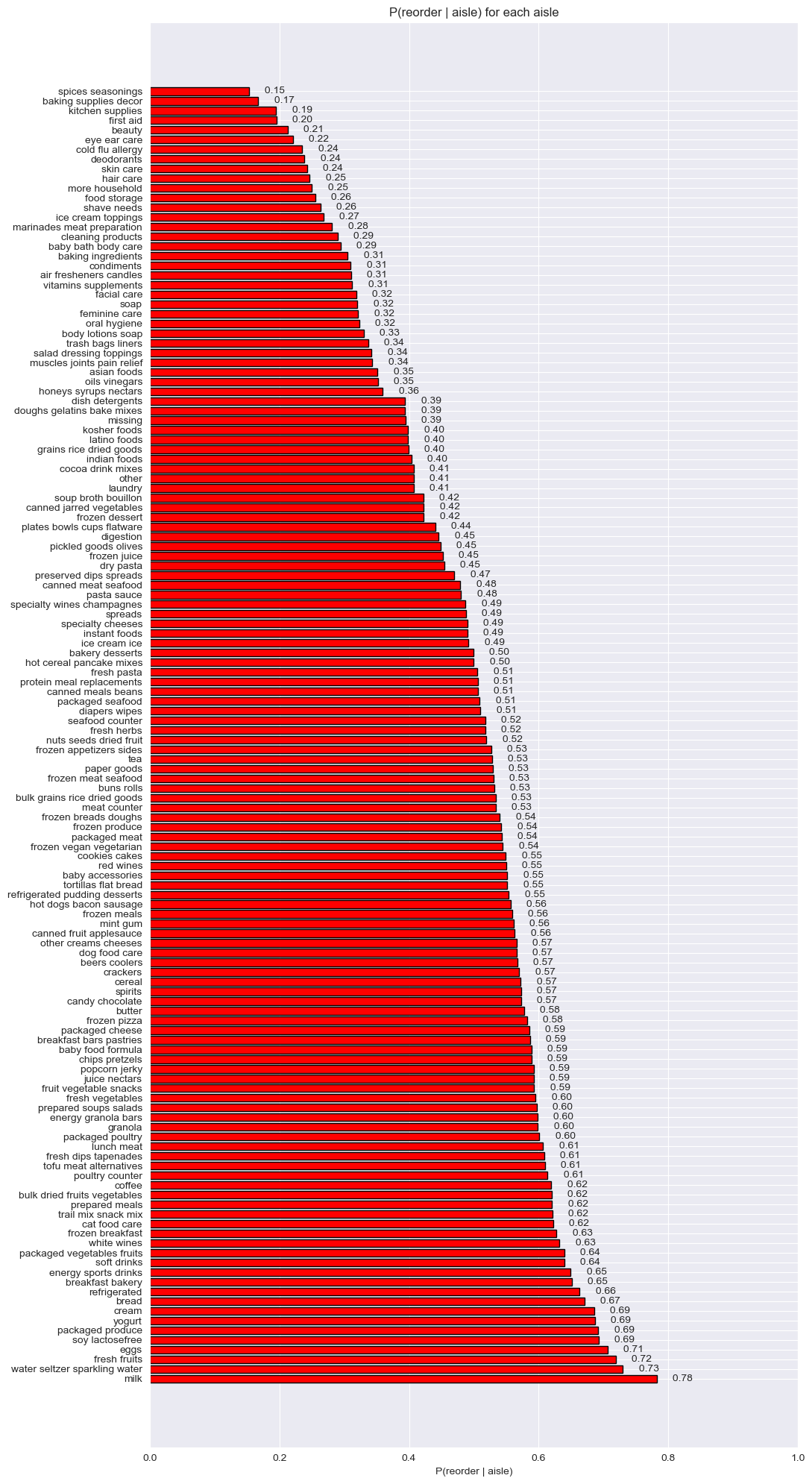
Probability of Reorder by Aisle
Drilling down to the aisle level (~134 aisles) shows even finer granularity:
\[
P(\text{reorder} \mid \text{aisle} = a) = \frac{\#\text{reorders from } a}{\#\text{purchases from } a}
\]
Probability of reorder from each aisle
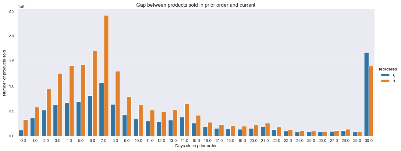
Impact of Order Gap on Reorder Behavior
The time between consecutive orders (days_since_prior_order) significantly influences reorder behavior. Data shows clear spikes at 7 days (weekly shoppers), with additional modes at 14 and 30 days.
Gap between orders and reorder behavior
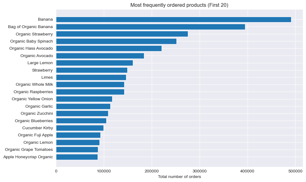
Most Popular Products
The top 20 most-ordered products are dominated by fresh produce — bananas, organic strawberries, and baby spinach lead by a wide margin. The heavy-tailed distribution means the top 10% of products account for roughly 50% of all order lines.
Top 20 most frequently ordered products
Cart Position Analysis
The median add-to-cart position distribution shows most products are added early — customers start with habitual items and then explore.
Distribution of median cart position across products
Feature Engineering
Several features are engineered at the user, product, and order level to encode the patterns uncovered above.
User-Level Features
Each user’s reorder tendency is quantified as the fraction of their total purchases that are reorders:
Before modeling, a quick signal assessment identifies which predictors carry meaningful information:
Show code
# Pearson correlation for numeric featuresnum_feats = ['order_number', 'order_dow', 'order_hour_of_day','days_since_prior_order', 'cart_size']numeric_corr = { feat: cart_df[feat].corr(cart_df['reordered'])for feat in num_feats}# Signal strength for categorical featurescat_feats = ['aisle_id', 'department_id']cat_signal = []for feat in cat_feats: rates = df.groupby(feat)['reordered'].mean() cat_signal.append({'feature': feat,'num_categories': rates.size,'std_of_rates': rates.std(),'range_of_rates': rates.max() - rates.min() })
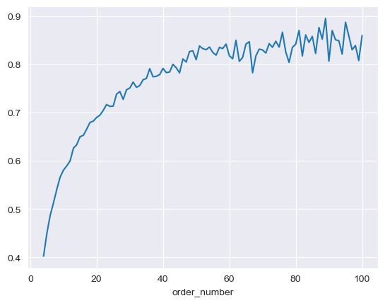
Reorder Rate vs Order Number
As users place more orders, their reorder rate climbs initially and then plateaus — confirming that customers develop stable purchasing habits over time.
Reorder rate as a function of order number
The Math Behind the Models
Problem 1: Will This Product Be Reordered?
For each observation \(n\) (a user–product pair in an order), define \(y_n \in \{0,1\}\) as the binary reorder indicator. A standard logistic regression models the probability as:
This assumes a single intercept \(\alpha\) and shared slopes \(\boldsymbol{\beta}\) across all users and products. The problem: User A (who reorders 90% of the time) and User B (who reorders 20% of the time) are forced to share the same baseline. Similarly, bananas and birthday candles get no product-specific adjustment.
The Hierarchical Extension
A hierarchical model introduces random effects — per-user and per-product intercept offsets drawn from population-level distributions:
Each user’s and product’s effect is pulled toward the global mean, with the degree of shrinkage controlled by \(\sigma_u^2\) and \(\sigma_p^2\). Users with abundant data get estimates closer to their individual rates; users with sparse data borrow strength from the population.
Problem 2: How Many Items in the Cart?
For each order \(i\), the cart size \(c_i\) (a non-negative integer) is modeled with a Poisson distribution and log-link:
This gives not just a point estimate but a complete probability distribution over cart sizes, enabling credible intervals for inventory planning and staffing decisions.
Prior Justification
Given the logistic scale and standardized predictors, weakly informative priors are used for all parameters:
Hierarchical Logistic Regression
\[
\alpha \sim \mathcal{N}(0, 1) \qquad \text{(global intercept)}
\]\[
\sigma_u, \sigma_p \sim \text{Half-}\mathcal{N}(0, 1) \qquad \text{(controls how far users/products stray from global intercept)}
\]\[
\tilde{u}, \tilde{p} \sim \mathcal{N}(0, 1) \qquad \text{(raw offsets for non-centered form)}
\]\[
\beta_{\text{num}}, \beta_{\text{dow}}, \beta_{\text{hour}} \sim \mathcal{N}(0, 1) \qquad \text{(fixed slopes)}
\]
On the logit scale, a \(\mathcal{N}(0,1)\) prior places most mass within \(\pm 2\), corresponding to probabilities between roughly 12% and 88%. This is broad enough to accommodate diverse effects without letting the model converge on extreme or implausible values. The half-normal priors on \(\sigma_u\) and \(\sigma_p\) regularize the group-level variation, shrinking sparse groups toward zero.
Poisson Regression
\[
\beta_0, \beta_1, \beta_2, \beta_3, \beta_4 \sim \mathcal{N}(0, 1) \qquad \text{(all coefficients on the log scale)}
\]
Non-Centered Parameterization
For computational efficiency, the hierarchical model uses a non-centered parameterization. Instead of sampling \(\gamma_u \sim \mathcal{N}(0, \sigma_u)\) directly, a standard normal auxiliary variable \(\tilde{u}\) is sampled and then scaled:
This is mathematically equivalent but breaks the correlation between \(\sigma_u\) and \(\gamma_u\) in the posterior — dramatically improving sampling efficiency when the number of groups (users, products) is large.
Model 1: Hierarchical Logistic Regression in Stan
Preparing the Data
Show code
df = order_products_train.merge( orders[['order_id', 'user_id', 'order_number', 'order_dow', 'order_hour_of_day']], on='order_id').merge( products[['product_id', 'aisle_id', 'department_id']], on='product_id')# Sample for tractable MCMCdf = df.sample(n=5000, random_state=42)# Integer indices for random effects (Stan 1-based)model_l = df[['user_id', 'product_id', 'order_number','order_dow', 'order_hour_of_day', 'reordered']].copy()model_l['user_idx'] = model_l['user_id'].astype('category').cat.codesmodel_l['product_idx'] = model_l['product_id'].astype('category').cat.codes
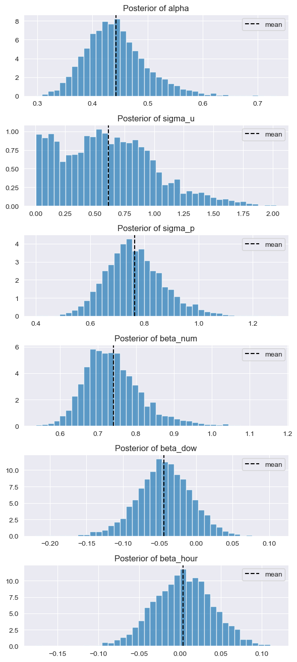
The posterior draws for the global parameters and fixed slopes reveal how much of the reorder variation is attributable to users, products, and order context:
Posterior distributions of α, σ_u, σ_p, β_num, β_dow, β_hour
Each posterior distribution tells a specific story about how Instacart customers behave. The histograms above show the density of 4,000 MCMC draws (4 chains × 1,000 samples) for each parameter. The dashed vertical line marks the posterior mean.
Global Intercept — \(\alpha \approx 0.44\)
The global intercept represents the baseline log-odds of reorder when all predictors are at their mean and user/product random effects are zero. Converting to probability through the logistic function:
This means an average user buying an average product has roughly a 61% chance of reordering it — closely matching the 59% overall reorder rate observed in the raw data. The tight posterior (narrow histogram) indicates high confidence in this estimate.
User-Effect Standard Deviation — \(\sigma_u \approx 0.62\)
This parameter controls how much individual users deviate from the global intercept. A value of 0.62 means users’ log-odds intercepts are drawn from \(\mathcal{N}(0, 0.62^2)\). To understand the practical impact, convert to odds ratios:
This means the most habitual users have reorder odds 3.4× the baseline, while the most exploratory users have odds just 0.3× the baseline. The wide spread confirms massive user heterogeneity — exactly the kind of variation that a flat model would miss.
Product-Effect Standard Deviation — \(\sigma_p \approx 0.75\)
Products vary even more than users. The 95% interval of product odds ratios spans:
A staple like whole milk has a strongly positive \(\delta_p\), pushing its reorder odds to 4× the baseline. A novelty item like a seasonal candle has a strongly negative offset, dropping to 0.23× the baseline. This asymmetry between products is the main reason hierarchical modeling outperforms flat approaches.
Order Number Slope — \(\beta_{\text{num}} \approx 0.75\)
One standard deviation increase in the user’s order count multiplies the odds of reorder by:
Experienced users are about twice as likely to reorder. This aligns with the EDA finding that reorder rates climb with order count before plateauing — the model has learned this relationship directly from the data.
The posterior is centered just below zero. Converting: \(\exp(-0.05) = 0.951\), indicating a 5% drop in odds per SD increase in day-of-week. This is a negligible effect — whether someone orders on a Monday or Saturday barely changes their reorder tendency.
The posterior density straddles zero almost symmetrically, confirming that hour of day has no measurable effect on reorder probability. Morning shoppers and late-night browsers reorder at the same rates.
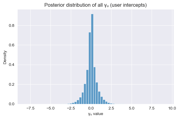
User and Product Random Effects
The distributions of per-user and per-product random intercepts show how the model captures individual-level variation:
Posterior distribution of all user random intercepts γᵤ
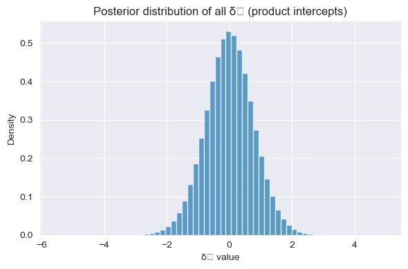
Posterior distribution of all product random intercepts δₚ
Show code
# User interceptsgamma_cols = [c for c in df_draws.columns if c.startswith('gamma_u[')]all_gamma = df_draws[gamma_cols].values.flatten()plt.figure(figsize=(6, 4))plt.hist(all_gamma, bins=60, density=True, alpha=0.7)plt.title("Posterior distribution of all γᵤ (user intercepts)")plt.xlabel("γᵤ value")plt.show()# Product interceptsdelta_cols = [c for c in df_draws.columns if c.startswith('delta_p[')]all_delta = df_draws[delta_cols].values.flatten()plt.figure(figsize=(6, 4))plt.hist(all_delta, bins=60, density=True, alpha=0.7)plt.title("Posterior distribution of all δₚ (product intercepts)")plt.xlabel("δₚ value")plt.show()
Prediction: Reorder Probability for a Specific User–Product Pair
To compute the probability that a specific user will reorder a specific product on their next order, the posterior draws are used directly:
Example result: For user 1235 and product 563, the posterior mean reorder probability is 0.977 with a 95% credible interval of [0.899, 0.999]. The model is highly confident this user will reorder this product.
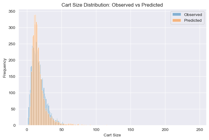
Model 2: Bayesian Poisson Regression for Cart Size
The second model shifts focus from what goes into the cart to how many items go in. For each order \(i\), the cart size \(c_i\) is modeled as:
Example result: For a user with average cart size 12.3, placing their 5th order on a Wednesday at 3 PM: expected cart size = 12.01 items, 95% predictive interval = [6, 19] items, and the probability of exactly 10 items is 0.105.
While classical models achieve competitive point metrics, only the Bayesian models deliver full posterior distributions over predictions. This means calibrated uncertainty estimates — credible intervals for reorder probability and cart size — that are essential for downstream decisions like inventory stocking, staffing, and personalized promotions.
Key Takeaways
1. Reorder behavior dominates the Instacart ecosystem. With 59% of all cart items being reorders, customer behavior is deeply habitual. The hierarchical model’s global intercept of \(\alpha \approx 0.44\) translates to a baseline reorder probability of 61%, confirming that the average user–product interaction leans toward repurchase. This makes reorder prediction a high-signal problem with direct commercial value for recommendation engines and inventory systems.
2. User and product heterogeneity demand a hierarchical approach. The posterior estimates of \(\sigma_u \approx 0.62\) and \(\sigma_p \approx 0.75\) reveal that both users and products contribute substantial variation beyond what fixed effects can capture. 95% of users fall within an odds-ratio range of \([0.30, 3.39]\), while products span \([0.23, 4.35]\). A flat logistic regression ignores this structure entirely, producing miscalibrated predictions for anyone who deviates from the population average.
3. Experience drives loyalty, not timing. The order number slope \(\beta_{\text{num}} \approx 0.75\) shows that experienced users are about twice as likely to reorder (\(\text{OR} = 2.12\)), while day-of-week (\(\beta_{\text{dow}} \approx -0.05\)) and hour-of-day (\(\beta_{\text{hour}} \approx 0\)) have negligible effects. This suggests that marketing efforts should focus on retention and building purchase history rather than optimizing delivery time slots.
4. Full predictive distributions enable risk-aware operations. The Bayesian Poisson model produces not just a point estimate for cart size but a complete probability distribution — enabling credible intervals like \([6, 19]\) items for a typical order. This tail-risk information is critical for warehouse staffing, delivery capacity planning, and inventory allocation, where underestimating demand is costly.
5. Partial pooling rescues sparse data. Many users and products have limited interaction histories. The hierarchical structure pools information across similar groups, producing stable estimates even for rare items and cold-start users. This is the practical advantage of the Bayesian framework over tree-based or flat classifiers — more reliable predictions exactly where they matter most.
6. Non-centered parameterization is essential at scale. With thousands of users and products, the naive centered parameterization creates a funnel geometry in the posterior that Stan’s NUTS sampler struggles with. The non-centered reparameterization — sampling \(\tilde{u} \sim \mathcal{N}(0,1)\) and computing \(\gamma_u = \tilde{u} \cdot \sigma_u\) — eliminates divergent transitions and yields clean, well-mixed chains.
NoteFull Project Report
For a complete writeup covering methodology, convergence diagnostics, model comparison tables, and future directions, download the full report: